threadlocalmutex.com

In any dimension, the key for an efficient implementation of a coordinate <=> Hilbert curve index mapping is finding a sequence of machine instructions that computes the subcube transformation group of that curve. In particular, if the transformation group multiplication can be represented as a logic circuit, the coordinate <=> Hilbert mapping algorithm can be modified to operate in time logarithmic in the number of bits per coordinate by using bitwise operations and prefix scans at the native register width to massively parallelize the logic circuit.

For this logarithmic algorithm, the Hilbert index => coordinate mapping is straightforward, while the reverse direction to find the Hilbert index given a coordinate tuple requires tracking all possible parent transformation, increasing complexity by a factor of the transformation group's order.

While in every dimension the transformation group is simply some (integer) subgroup of the orthogonal rotation group $O(d)$, clearly this is not a very compact representation, requiring a quadratic number of bits as d increases.

In low dimensions, a compact representation of the transformation group can found through rather tediuos manual geometric or combinatorial work. See previous work http://threadlocalmutex.com/?p=126, http://threadlocalmutex.com/?p=157. While the group in two dimensions (isomorphic to the Klein group V) is trivially representable as a pair of XOR-operations, we find that in three dimensions the group (isomorphic to the alternating group A4) is already quite challenging to represent efficiently as logic circuits. Furthermore, there is no obvious connection between V and A4 that would allow us to extrapolate a possible choice in higher dimensions.

To extend this work to higher dimensions, it's clear the previous manual approach is untenable. Instead, let us try to derive from scratch a recursive definition of higher dimensional Hilbert curves. This will yield an efficient representation of the transformation group in every dimension, from which one can easily derive a log(n) time implementation in 4 dimensions. The general result here matches other treatments of the subject by Butz or Lawder, but we will nevertheless derive it without consideration of prior work in order to solely keep the focus on implementation efficiency.

Before we begin, some comments on the uniqueness of the Hilbert curve in various dimensions are in order. In 2D, the shape of the Hilbert curve is uniquely defined up to similarity (i.e., rotation or reflection). In 3D, there are already 1536 curves unique up to similarity, comprising 6 base curves with 256 subvariants each, each of which flips the spatial orientation for some subset of the 8 octants. Typically the first of those 1536 (in the order listed by Alber and Niedermeier, On Multi-dimensional Hilbert Indexings) is implemented as "the" 3D Hilbert curve. However, we can fix both the base shape of the curve as well as choice of transformation group for each subcube in a way that yields a "canonical" Hilbert curve.

Existing implementations in 2D and 3D typically provide a curve that starts the base curve at (y, x) = (0, 0) resp. (z, y, x) = (0, 0, 0) and ends at (y, x) = (0, 1) resp (z, y, x) = (0, 0, 1). However, for the general construction, it is more convenient to have the base level curve end at the highest coordinate index; i.e., (y, x) = (1, 0) resp. (z, y, x) = (1, 0, 0), which allows recursively composing the base curve to higher dimensions. The difference between the composable and standard variants corresponds to a simple rotation of the coordinate tuples.

To construct the base level curve for dimension d, we start by embedding the base curve of dimension d - 1, which traverses from (0, …, 0) to (0, 1, 0, …, 0), then move into the new dimension (1, 1, 0, …, 0), followed by another copy of the lower dimension curve traversing backwards to (1, 0, 0, …, 0). his constructions matches exactly the construction of a d-bit Gray code via reflections, so we can express the mapping between index tuple and corresponding coordinate tuple as

x(I) = binary2gray(I)
     = I ^ (I >> 1)

This Gray code traversal corresponds to the first of the 6 base level curves in Alber and Niedermeier's work, and is the same construction used by Butz and Lawder in higher dimensions.

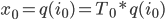
Now for each of the subcubes along this traversal, we want to apply a transformation that allows mapping the "base edge" of each cube (0, 0, …, 0) -> (1, 0, …, 0), which defines its curve start and end point, to an arbitrary edge defined by transformed start end and points s(I) -> e(I). If we uniquely define how the base edge should be transformed, the transformation of the remainining hypercube vertices follows naturally. In 2D and 3D, we achieved this through rotations about interior diagonals passing through the cube's center. The same concept can be applied in higher dimensions as well.

We can see that a rotation around the cube's "main" interior diagonal (the diagonal from the origin to the far end (0, 0, …, 0) -> (1, 1, …, 1)) that maps cube corners back to cube corners corresponds to a cyclic rotation of the bits representing a cube coordinate, which we'll express x' = x <<< n. For example, for d = 3, a rotation around the axis (0, 0, 0) -> (1, 1, 1) by an angle of 360/d degrees corresponds to a cyclic coordinate shift (x, y, z) -> (y, z, x).

To represent rotations around an other interior diagonals, note that we can first reflect the rotation diagonal to the main diagonal, rotating around the main diagonal, and then performing the same reflection again (its own inverse!) to map back to the chosen diagonal. Expressed in bit log, icif s is one of the two vertices of an interior diagonal, we have

x' = ((x ^ s) <<< n) ^ s
   = (x <<< n) ^ (s ^ (s >>> n))

Note that the second term (s ^ (s >>> n)) has even parity, and that every bit pattern with even parity can be represented in this form. Thus the group of rotations about interior diagonals is isomorphic to cyclic rotations of the coordinates followed by a even number of reflections of coordinate axes:

x' = (x <<< n) ^ c

where n in [0… d), c in [0..2^d) with parity(c) = 0. It's easy to verify this operation actually forms a group of order d*2^(d-1) which maps fairly well to machine instructions.

Because the parity of c is even, the transformation always includes an even number of reflections, meaning the orientation of each subcube is preserved. In the 3D case, this corresponds to fixing the choice to the first of the 256 subvariants; all 255 others do not preserve orientation. This transform also fulfills our requirement that we find a unique pair (n, c) that transforms the base edge to an arbitrary edge s -> e, which lets us uniquely define a subcube's transformation just from its positioning of the base edge:

(0 <<< n) ^ c = s
((1<<(d-1)) <<< n) ^ c = e

From which follows:

c = s
n = ctz(s^e) + 1

Where ctz(x) counts the number of trailing zeroes in the binary representation of x. Although s ^ e is always a non-zero power of two if we chose two vertices directly connected by an edge, we'll define ctz(0) = -1 by convention for later simplification.

This completes that this group construction is indeed suitable for higher dimensional Hilbert subgroups, and in fact, one can verify that this matches the group structure for our manually derived low-dimensional curves. What still remains is finding explicit formulas for s(I) and e(I) for a given Hilbert curve index I; that is, finding an edge traversal that we can use to align the next level of subcubes. The transformation group follows uniquely from this choice.

Since the edge traversal must be connected, the start s(I) of a cube is determined by the end e(I-1) of the previous one:

s(0) = 0
s(I) = e(I - 1) ^ binary2gray(I) ^ binary2gray(I - 1)

Expanding in terms of the the edge vectors s(I) ^ e(I) gives an inductive formula for s(I):

s(I) = e(I - 1) ^ binary2gray(I) ^ binary2gray(I - 1)
     = binary2gray(I) ^ (s(I - 1) ^ e(I - 1)) ^ ... ^ (s(0) ^ e(0))

Now the direction of each edge s(I) ^ e(I) can be constructed again by a recursive formulation similar to the main cube ordering. We can find that in 2D, the edge pattern is "x, y, y, x", and in 3D "x, y, y, z, z, y, y, x". Recursively, we can extend the pattern by duplicating it and replacing the middle pair by an edge into the next higher dimension. In 4D, this yields "x, y, y, z, z, y, y, w, w, y, y, z, z, y, y, x". We can find this is expressible as

s(I) ^ e(I) = 1 << ctz(binary2gray(I) &amp; ~(1 << (d - 1)) + 1)

where we're making use of the convention ctz(0) = -1. The combined XOR of these terms yields the pattern "0, 1, 3, 1, 5, 1, 3, 1, 9, 1, 3, 1, 5, 1, 3, 1" for s(I) ^ binary2gray(I) in 4D, which we can concisely generalize as

s(0) = 0
s(I) = binary2gray(I) ^ ((1 << ctz(I)) | 1)
     = binary2gray(I) ^ (I &amp; -I | 1)

using the trick that I & -I isolates the least set bit of I.

Putting these all together, this yields an algorithm for transforming from Hilbert curve index to Morton in arbitrary dimensions that maps reasonably well to machine instructions:

uint32_t rol(uint32_t x, uint32_t bits, uint32_t n)
{
    assert(bits < n);
    return ((x << bits) &amp; ((1U << n) - 1)) | (x >> (n - bits));
}

uint32_t ror(uint32_t x, uint32_t bits, uint32_t n)
{
    assert(bits < n);
    return ((x << (n - bits)) &amp; ((1U << n) - 1)) | (x >> bits);
}

uint32_t ctz(uint32_t x)
{
    // Replace with compiler intrinsic of choice
    unsigned long index;
    return _BitScanForward(&amp;index, x) ? index : -1;
}

uint32_t hilbertToMortonN(uint32_t index, uint32_t dim, uint32_t bits)
{
    uint32_t c = 0;
    uint32_t n = 0;

    uint32_t mask = (1U << dim) - 1;
    uint32_t hibit = 1U << (dim - 1);

    uint32_t morton = 0;

    for (uint32_t i = 0; i < bits; ++i)
    {
        uint32_t I = mask &amp; (index >> (dim * (bits - i - 1)));

        uint32_t gray = I ^ (I >> 1);

        uint32_t M = rol(gray, n, dim) ^ c;
        morton = (morton << dim) | M;

        uint32_t N = 2 + ctz(gray &amp; ~hibit);
        uint32_t C = I == 0 ? 0 : gray ^ (I &amp; -int32_t(I) | 1);

        c = rol(C, n, dim) ^ c;
        n = (n + N) % dim;
    }

    return morton;
}

The inverse is found by inverting each operation in the loop:

uint32_t mortonToHilbertN(uint32_t morton, uint32_t dim, uint32_t bits)
{
    uint32_t c = 0;
    uint32_t n = 0;

    uint32_t mask = (1U << dim) - 1;
    uint32_t hibit = 1U << (dim - 1);

    uint32_t index = 0;

    for (uint32_t i = 0; i < bits; ++i)
    {
        uint32_t M = mask &amp; (morton >> (dim * (bits - i - 1)));

        uint32_t gray = ror(c ^ M, n, dim);

        uint32_t I = gray2integer(gray);

        index = (index << dim) | I;

        uint32_t N = 2 + ctz(gray &amp; ~hibit);
        uint32_t C = I == 0 ? 0 : gray ^ (I &amp; -int32_t(I) | 1);

        c = rol(C, n, dim) ^ c;
        n = (n + N) % dim;
    }

    return index;
}

Up to changing the order of coordinates, this yields the same result as the 2D and 3D algorithms previously published here. Roughly this method is O(n*d), if we allow for dimensions d larger than the native word size, however specializations for specific d should yield significant improvements by eliminating the modulo operation which is comparably slow even on modern architectures unless optimized for some constant.

To implement the log time version of mapping from Hilbert to Morton index hinted at earlier, we now need to supply logic circuits for the main ingredients of the transformation group; that is, cyclic addition of order d and d-bit rotation, as well as some minor bits connective tissue.

Of these, bit rotation is relatively straightforward to represent in circuit logic as a barrel shifter of size O(d*log(d)). This causes complexity to increase from O(d*n) for the linear time implementation to at least O(d*log(d)*log(n)) for the version logarithmic in the bit count; similarly the connective tissue increases complexity, although I have not performed a precise analysis. The main challenge for providing an optimized version for a fixed d however lies in a cyclic addition circuit. When d is a power of two, this is simply a log(d)-bit adder circuit, as we can discard overflow bits. For non-powers-of-two however this circuit is much more complex, which in hindsight somewhat explains the difficulty in constructing an efficient version of it for 3 dimensions. Thus useful candidates for dimensions in which we could expect efficiency gains compared to the linear time version would be (2, 4, 8, 16, …). Clearly one could provide a generic version that works for abitrary d, but constructing the logic circuits on the fly by far outweighs the actual computation performed by the linear time mapping.

Finally, I will present such an implementation for 4 dimensions, where significant work has gone into optimizing the circuits by hand to exploit various symmetries (ss usual, replace pdep and other intrinsics as needed):

uint32_t hilbertToMorton4(uint32_t index, uint32_t bits)
{
    // Extract index tuples and align to MSB
    uint32_t i0 = _pext_u32(index, 0x11111111) << (32 - bits);
    uint32_t i1 = _pext_u32(index, 0x22222222) << (32 - bits);
    uint32_t i2 = _pext_u32(index, 0x44444444) << (32 - bits);
    uint32_t i3 = _pext_u32(index, 0x88888888) << (32 - bits);

    // Gray code
    uint32_t gray0 = i0 ^ i1;
    uint32_t gray1 = i1 ^ i2;
    uint32_t gray2 = i2 ^ i3;
    uint32_t gray3 = i3;

    // Initial subcube rotations
    uint32_t n0 = (gray0 | ~gray1 &amp; gray2) >> 1;
    uint32_t n1 = (~gray0 &amp; (gray1 | gray2)) >> 1;

    // Prefix sum of subcube rotations
    for(uint32_t shift = 1; shift <= 4; shift *= 2)
    {
        uint32_t s0 = (n0 >> shift) | (~0u << (32 - shift));
        uint32_t s1 = (n1 >> shift) | (~0u << (32 - shift));

        uint32_t r0 = ~(s0 ^ n0);
        uint32_t r1 = (s0 | n0) ^ (s1 ^ n1);

        n0 = r0;
        n1 = r1;
    }

    // Map curve indices to flip bits
    uint32_t c0 = gray0 ^ (i0 | i1 | i2 | i3);
    uint32_t c1 = gray1 ^ (~i0 &amp; i1);
    uint32_t c2 = gray2 ^ (~i0 &amp; ~i1 &amp; i2);
    uint32_t c3 = gray3 ^ (~i0 &amp; ~i1 &amp; ~i2 &amp; i3);

    // Rotate and accumulate flip bits
    uint32_t g0 = gray2integer(c0 ^ (n0 &amp; (c0 ^ c3)) ^ (n1 &amp; (c0 ^ c2)));
    uint32_t g1 = gray2integer(c1 ^ (n0 &amp; (c1 ^ c0)) ^ (n1 &amp; (c1 ^ c3)));
    uint32_t g2 = gray2integer(c2 ^ (n0 &amp; (c2 ^ c1)) ^ (n1 &amp; (c2 ^ c0)));

    // Rotate and flip coordinates
    uint32_t X = gray0 ^ (n0 &amp; (gray0 ^ gray3)) ^ (n1 &amp; (gray0 ^ gray2 ^ (n0 &amp; i0))) ^ (g0 >> 1);
    uint32_t Y = gray1 ^ (n0 &amp; (gray1 ^ gray0)) ^ (n1 &amp; (gray1 ^ gray3 ^ (n0 &amp; i0))) ^ (g1 >> 1);
    uint32_t Z = gray2 ^ (n0 &amp; (gray2 ^ gray1)) ^ (n1 &amp; (gray2 ^ gray0 ^ (n0 &amp; i0))) ^ (g2 >> 1);

    // Recover W from symmetry conditions
    uint32_t W = X ^ Y ^ Z ^ i0;

    // Shift back from MSB
    X >>= (32 - bits);
    Y >>= (32 - bits);
    Z >>= (32 - bits);
    W >>= (32 - bits);

    // Compose to Morton code
    return
        _pdep_u32(X, 0x11111111) |
        _pdep_u32(Y, 0x22222222) |
        _pdep_u32(Z, 0x44444444) |
        _pdep_u32(W, 0x88888888);
}

In contrast, a logarithmic version of the reverse mapping from Morton to Hilbert curve, as was already implemented for 2D, causes a complexity blow up in the order of the transformation group for simultaneously transforming a set of possible paths for each group element, bringing us to at least O(d*log(d)*2^d*log(n)). Since the two dimensional logarithmic algorithm is already just barely faster in practice than the linear one, which was only achieved through heavy manual optimization, it is unlikely that any higher dimensional instances of this algorithm will be efficient enough, implementation complexity notwithstanding. Thus the 4D version given here will likely be the last O(log(n)) algorithm I will publish.

I'm happy to announce that my software rasterizer side project has been picked up by a major commercial VR product a while ago. While I can't go into too much detail, adding in the rasterizer gave an average frame time saving of 1ms on the CPU and GPU each, which was critical to shipping the product on the targetted min spec configuration. There's some unique challenges in using this in practice which I'm going to address as part of this post, as well as going into some details regarding the next release of the rasterizer which brings a ~1.5x speedup compared to the initial release. Because real life has forced me to delay this post a bit, it covers both commits https://github.com/rawrunprotected/rasterizer/commit/d2fa65fd6b5df8b94d8d4b02914354c9aca2d46d and https://github.com/rawrunprotected/rasterizer/commit/ca469a402a65341a37c692ed06b4d355fe6d5494, even those are almost a year apart.

Over-occlusion in VR

Using software occlusion culling in 3D graphics typically involves some amount of false negatives; i.e. queries returning that an object is occluded even though it should be visible on screen. The reason for that is that software rasterization is generally performed on a lower resolution than the target render resolution. Unless the rasterizer is written "to spec" and matches the behavior of the hardware graphics API exactly, it may also introduce additional error through differences in vertex quantization or edge test precision.

This isn't much of a problem in practice for flat-screen applications as long as the incorrect over-occlusion can be kept below some threshold, say 5 pixels, which is barely noticeable to the user. In VR however, lens distortion implies that angular resolution is much lower, particularly in the center of the screen. This makes even small over-occlusion artifacts very noticable. Another problem is that it's not practical to perform occlusion for both eyes each frame, and it is easy to construct cases where culling only for one eye or a synthetic camera position centered between the eyes fails completely. Applying occlusion culling naively led to some user complaints in the initial beta release of the product as there were some geometric constellations which would result in noticable artifacts.

A simple approach to both of these issues is to apply a simple form of temporal filtering. For monoscopic rendering, applying a small amount of sub-pixel camera jitter helps break quantization errors. The jitter pattern repeats over a small period N (e.g. 4 frames), and an object is only considered culled when occlusion queries fail for all N of these frames. The standard MSAA sample distributions work well in practice as jitter patterns. This is fairly cheap to implement by means of a simple counter per object. While it has the disadvantage of introducing a small delay before objects can be culled, it solves the false negative problem for all practical purposes even when downscaling the target resolution by a factor of 5 in both X and Y.

The same can then be extended to stereoscopic rendering, by culling against left and right eye in alternating frames; doubling the effective length of the jitter period. As this is effectively fully external to the usage of the rasterizer and I'm not at liberty to publish the code anyway, I won't include the temporal filtering approach in the public release.

Another source of errors occurs when the camera moves close enough to near-clip the geometry. While this should ideally be prevented on a higher level as in can result in comfort issues in VR, it produces artifacts as the rasterizer does not perform near-clipping, which allows the user to peek through geometry and see objects flickering in and out of existence. As full emulation of near-clipping is infeasible for performance reasons, a simple hack solves this problems: Pixels which are in front of the near plane are clamped to depth values of 0xFFFF by the rasterizer, so simply adding 1 to each value forces these pixels to wrap around to the far plane, effectively discarding them. The near resulting clipping edge doesn't fully match the GPU result, but is good enough to avoid major discrepancies.

Now for the optimizations in the latest version:

Triangle setup optimizations

The first version of the rasterizer required AVX2, but performed vertex transform and triangle setup only at SSE widths (i.e. 4 in parallel). This has been extended to the full AVX vector width so that 8 triangles are set up in parallel, and the vertex packing format has been adapted accordingly. This results in a rather modest performance increase as it reduces the average utilization per vector, since it's much less likely to discard an entire batch of triangles via back face culling, but it's a net win overall.

An interesting trick was to remove most of the masking on decoding vertices from the packed 11/11/10 vertex format which shaves of a few instructions in the vertex transform portion. For transforming the X component, rather than right-shifting to remove the Y and Z component, I'm now applying the equivalent scale of 1.0f / (1u << 21) as part of the projection matrix. This result in some bleedover of the Y and Z components that were previously masked out, into the X component, so the meshes end up slightly skewed. This effect however can be cancelled by applying the inverse skew to the projection matrix. Making use of the _mm256_broadcast_ss allows keeping most of the projection matrix in memory, which reduces register pressure during the vertex transformation. The rest of the triangle setup code has received a bit of cycle shaving by moving around constant factors, so that the entire portion that translates the edge equations into block space is now removed.

Advanced transposition

A side effect of the wider triangle setup is that transposing the data from triangle-parallel to pixel-parallel layout becomes much harder, as AVX shuffle operations typically operate on each sub-lane of 4 elements separately. This implies having to extract and store each lane to memory separately. However, we can also restrict the shuffle operations to be incomplete, and store data to memory without the full sequence of operations, which effectively changes the order of triangles within each batch. Modifying the primitive index lets us iterate over the triangles in each batch in a changed order, but saving quite a few instructions for transposition.

Fully unrolled coverage mask generation

Similar to the triangle setup, the critical inner loop code was restricted to 4-wide SSE. The main obstacle to widening this was the fact that the _mm256_packus_epi32 operation did not operate on 8 lanes in parallel, resulting in some unintentional interleaving. This was fixed by pre-applying a permutation to each rasterization table entry, allowing the transfer from a single 64bit mask to 4 16x16bit depth masks in a few instructions.

 

Fast clears

This is a simple optimization employed by virtually every hardware rasterizer. Rather than resetting the full-resolution depth buffer to the far plane, we only mark blocks as cleared, which saves significant amounts of bandwidth. Before the previously mentioned unrolled coverage mask generation, this didn't yield much benefit, but now allows squeezing out a few extra percentage points. Since we can't afford an extra buffer to store tile metadata, fast cleared blocks are marked in the HiZ buffer with the value 1. This value is extraordinarily unlikely to be generated during normal operation (compared to using HiZ == 0 which happens all the time), and close enough to 0 so we can ignore falsely culled blocks.

Effectively this change allows us to skip the prior depth load for a large proportion of blocks at the cost of an additional branch for an overall net win. It requires some extra complexity for reading back full depth, but since that is intended for debug visualization only, we can ignore this impact.

 

Complete classification of rasterized quadrilaterals

Now for the meat of the actual original research work. As you may be aware, my rasterizer works with quads rather than triangles (which gives a net benefit as most meshes are authored as quads, which is trivial to recover from a trangle representation).

While convex quadrilaterals are mostly trivial to handle by simply adding a 4th edge equation, this is not the case as soon as non-convex or non-simple vertex quadrilaterals turn up. Until now, the rasterizer handled this with a 5th edge, which splits non-convex quads into two triangles, which are then composed separately. This occurs quite frequently in practice, even if the source data is fully comprised of convex quads, as vertex quantization and rounding errors during perspective projection can easily make any geometry a mess of concave or self-overlapping quads.

Unfortunately, this adds significant overhead for the 5th edge, as well has handling some cases incorrectly. To rectify this, I set out to systematically investigate the properties of possible quads. By exhaustively searching over all possible configurations, I found a total of 25 distinct vertex configurations (rather than the over-simplified 2 cases I handled before). The program I wrote for this breaks my personal complexity record - it is in a search error of , with a total nesting depth of 14 loops.

Describing the complete classification is out of scope for this post, but the important classes are the following ones:

• Culled - occurs for example if both triangles of the quad are backfacing, or in front of the W plane, or a mix of these.
• Convex - the obvious simple case.
• Triangle 0 or triangle 1 culled - the quad is "folded over" so that a single sub triangle is backface culled.
• Concave left or concave right - both sub triangles are forward facing, but with an angle > 180 degrees at either connecting vertex.
• Concave center - some vertices are in front of the camera plane so that the remaining edges form a sort of inifinite W shape, which is extremely rare (< 1 in 1e8 triangles).

All other classes are specialization but can be represented as subsets of these 7. Notably, each of these cases requires only 3 or 4 edge equations to evaluate the covered area, rather than the 5 previously used.

As each configuration can be described only by the signs of the areas of each sub triangle (4 bits including complementary areas) as well as the signs of the W component of each vertex (another 4 bits), a simple lookup table with 16 resp. 256 entries (if any W < 0) allows correctly categorizing each primitive. This lookup is expensive due to the high latency of the gather operation, but allows handling the backface culling and near plane culling tests at the same time, both of which are simply represented by specific entries in the LUT.

Inside the inner-most loop we need to switch over the primitive configuration to determine how to combine the bit masks for individual edge equations. Luckily, the distribution is heavily skewed, with convex primitives being much more likely than the single triangles, which in turn are an order of magnitude more likely to occur than the concave cases. Specializing heavily for the convex case wasn't possible before due to the incorrect handling of some cases, but now yields a significant performance gains. For example, we can now skip evaluation of the edge equations for the rest of a scan line once we enter and leave the covered primitive area.

...sort of.

The core of computing 2D coordinates from a Hilbert index in logarithmic time is a XOR prefix sum. As it so happens, the upper bits of carry-less multiplication with -1 are equivalent to a XOR prefix sum. On an x86 machine with CLMUL and PEXT support, this yields the following "constant time" algorithm for mapping a 32bit Hilbert index to 16bit X and Y:

void hilbertIndexToXY_constantTime(uint32_t i, uint32_t& x, uint32_t& y)
{
	uint32_t i0 = _pext_u32(i, 0x55555555);
	uint32_t i1 = _pext_u32(i, 0xAAAAAAAA);

	uint32_t A = i0 & i1;
	uint32_t B = i0 ^ i1 ^ 0xFFFF;

	uint32_t C = uint32_t(_mm_extract_epi16(_mm_clmulepi64_si128(_mm_set_epi64x(0, 0xFFFF), _mm_cvtsi32_si128(A), 0b00), 1));
	uint32_t D = uint32_t(_mm_extract_epi16(_mm_clmulepi64_si128(_mm_set_epi64x(0, 0xFFFF), _mm_cvtsi32_si128(B), 0b00), 1));

	uint32_t a = C ^ (i0 & D);

	x = (a ^ i1);
	y = (a ^ i0 ^ i1);
}

Of course this isn't really a constant time solution since the CLMUL intrinsic is limited to 64bit operands, and can't be extended to operate on bits in time in any reasonable machine model. In practice, this solution also tends to be a hair slower than the logarithmic time solution since both transferring data into/out of SSE registers and the CLMUL intrinsic itself are rather high latency operations.

Finally I've managed to implement an optimized version of the 3D Hilbert Index -> XYZ transform in logarithmic time. The crucial element was finding an efficient bitwise representation of the alternating group A4. In the end I decided for a rather direct representation as a subgroup of S4, describing each permutation as a 4-tuple (a,b,c,d). Multiplication in this form (implementing 32 operations at the same time bitwise SIMD style) is then a simple bit selection:

struct S4x32
{
  uint32_t a1;
  uint32_t a0;

  uint32_t b1;
  uint32_t b0;

  uint32_t c1;
  uint32_t c0;

  uint32_t d1;
  uint32_t d0;
};


S4x32 mul(S4x32 x, S4x32 y)
{
  S4 res;

  // If x.a == 0, let res.a = y.a; else if x.a == 1, let res.a = y.b; else if x.a == 2, let res.a = y.c, etc.
  res.a0 = (y.a0 & ~x.a0 & ~x.a1) | (y.b0 & x.a0 & ~x.a1) | (y.c0 & ~x.a0 & x.a1) | (y.c0 & x.a0 & x.a1);
  res.a1 = (y.a1 & ~x.a0 & ~x.a1) | (y.b1 & x.a0 & ~x.a1) | (y.c1 & ~x.a0 & x.a1) | (y.c1 & x.a0 & x.a1);
  res.b0 = (y.a0 & ~x.b0 & ~x.b1) | (y.b0 & x.b0 & ~x.b1) | (y.c0 & ~x.b0 & x.b1) | (y.c0 & x.b0 & x.b1);
  res.b1 = (y.a1 & ~x.b0 & ~x.b1) | (y.b1 & x.b0 & ~x.b1) | (y.c1 & ~x.b0 & x.b1) | (y.c1 & x.b0 & x.b1);
  res.c0 = (y.a0 & ~x.c0 & ~x.c1) | (y.b0 & x.c0 & ~x.c1) | (y.c0 & ~x.c0 & x.c1) | (y.c0 & x.c0 & x.c1);
  res.c1 = (y.a1 & ~x.c0 & ~x.c1) | (y.b1 & x.c0 & ~x.c1) | (y.c1 & ~x.c0 & x.c1) | (y.c1 & x.c0 & x.c1);
  res.d0 = (y.a0 & ~x.d0 & ~x.d1) | (y.b0 & x.d0 & ~x.d1) | (y.c0 & ~x.d0 & x.d1) | (y.c0 & x.d0 & x.d1);
  res.d1 = (y.a1 & ~x.d0 & ~x.d1) | (y.b1 & x.d0 & ~x.d1) | (y.c1 & ~x.d0 & x.d1) | (y.c1 & x.d0 & x.d1);

  return res;
}

This is a lot less code than the autogenerated transform code of the original proof of concept implementation. Now there's some further symmetries that we can immediately exploit. Since there are no duplicate values in a permutation tuple, the last element is uniquely determined by the remaining ones, via d = a ^ b ^ c, and we can get rid of two components.

Since we're in the subgroup A4, the third element also happens to be uniquely determined as we only allow even permutations. After some logic optimizations, we arrive at the rather compact

struct A4x32
{
  uint32_t a1;
  uint32_t a0;

  uint32_t b1;
  uint32_t b0;
};

A4x32 mul(A4x32 x, A4x32 y)
{
  A4x32 res;

  uint32_t yc1 = y.a0 ^ y.b0 ^ y.b1;
  uint32_t ys = y.a1 ^ y.b1;
  uint32_t yc0 = ~((ys & y.a0) ^ (~y.s & y.b0));

  res.a0 = (y.a0 & ~(x.a0 ^ x.a1)) ^ (y.b0 & x.a0) ^ (yc0 & x.a1);
  res.a1 = (y.a1 & ~(x.a0 ^ x.a1)) ^ (y.b1 & x.a0) ^ (yc1 & x.a1);
  res.b0 = (y.a0 & ~(x.b0 ^ x.b1)) ^ (y.b0 & x.b0) ^ (yc0 & x.b1);
  res.b1 = (y.a1 & ~(x.b0 ^ x.b1)) ^ (y.b1 & x.b0) ^ (yc1 & x.b1);

  return res;
}

With this key piece, implementing the remaining function is straightforward. After prefix scanning, we only need to bring the transforms back into a representation that allows us to efficiently transform each octant in 3D. Luckily it's relatively easy to convert from the representation as a permutation tuple to a 3D transformation matrix. Putting it all together, this is the result:

void hilbertTo3D_logarithmic(uint64_t hilbertIndex, uint32_t bits, uint32_t& x, uint32_t& y, uint32_t& z)
{
  // Deinterleave index bits - use a different method if pext is not available
  uint32_t i0 = _pext_u64(hilbertIndex, 0x9249249249249249ull << 0);
  uint32_t i1 = _pext_u64(hilbertIndex, 0x9249249249249249ull << 1);
  uint32_t i2 = _pext_u64(hilbertIndex, 0x9249249249249249ull << 2);

  // Align to MSB
  i0 <<= 32 - bits;
  i1 <<= 32 - bits;
  i2 <<= 32 - bits;

  // Compute initial transform from index
  uint32_t j = ~(i1 ^ i2);
  uint32_t ta1 = (i2 & ~i1 & i0) | (j & ~i0);
  uint32_t ta0 = i0 | i1 | i2;
  uint32_t tb1 = (~i2 & i1 & ~i0) | (j & i0);
  uint32_t tb0 = i2 & i1 & i0;

  // Shift downwards, filling MSB with identity transform
  ta0 >>= 1;
  ta1 >>= 1;
  tb0 = (tb0 >> 1) | 0x80000000;
  tb1 >>= 1;

  // Prefix scan iteration
  auto fold = [&](uint32_t shift)
  {
    // Shift downwards
    uint32_t sa0 = ta0 >> shift;
    uint32_t sa1 = ta1 >> shift;
    uint32_t sb0 = (tb0 >> shift) | (~0 << (32 - shift));
    uint32_t sb1 = tb1 >> shift;

    // Recover third element of permutation which is uniquely determined in A4 by the first two elements
    uint32_t sc1 = sa0 ^ sb0 ^ sb1;
    uint32_t ss = sa1 ^ sb1;
    uint32_t sc0 = ~((ss & sa0) ^ (~ss & sb0));

    // Multiply permutations
    uint32_t ra0 = (sa0 & ~(ta0 ^ ta1)) ^ (sb0 & ta0) ^ (sc0 & ta1);
    uint32_t ra1 = (sa1 & ~(ta0 ^ ta1)) ^ (sb1 & ta0) ^ (sc1 & ta1);
    uint32_t rb0 = (sa0 & ~(tb0 ^ tb1)) ^ (sb0 & tb0) ^ (sc0 & tb1);
    uint32_t rb1 = (sa1 & ~(tb0 ^ tb1)) ^ (sb1 & tb0) ^ (sc1 & tb1);

    // Store current transform
    ta0 = ra0;
    ta1 = ra1;
    tb0 = rb0;
    tb1 = rb1;
  };

  // Apply prefix scan
  fold(1);
  fold(2);
  fold(4);
  fold(8);
  fold(16);

  // Recover untransformed octants
  uint32_t o0 = i0 ^ i1;
  uint32_t o1 = i1 ^ i2;
  uint32_t o2 = i2;

  // Build transformation matrix columns from permutation
  uint32_t m0 = ~(ta1 ^ tb1);
  uint32_t m2 = ~(ta0 ^ tb0);
  uint32_t m1 = ~(m0 | m2);

  uint32_t ma = tb0 ^ m0;
  uint32_t mc = ta1 ^ m2;
  uint32_t mb = ~ta1 & ~ta0 & tb1 | ta1 & ta0 & ~tb1 | ~ta0 & tb1 & tb0 | ta0 & ~tb1 & ~tb0;

  // Apply transform to original octants
  x = (m0 & o0) ^ (m1 & o1) ^ (m2 & o2) ^ ma;
  y = (m2 & o0) ^ (m0 & o1) ^ (m1 & o2) ^ mb;
  z = (m1 & o0) ^ (m2 & o1) ^ (m0 & o2) ^ mc;

  // Undo MSB alignment
  x >>= 32 - bits;
  y >>= 32 - bits;
  z >>= 32 - bits;
}

The resulting code quite nicely demonstrates all of the symmetries inherent to the problem, so I consider it unlikely to find any further significant reductions to the bit logic. The instruction count per iteration is unfortunately still massive compared to the rather trivial O(n) version, so for small bit counts this method is slower in practice despite the lower asymptotic complexity. The cutoff point seems to be around transforming 63 -> 3x21 bits, where it starts being just barely faster on my machine. So for computing positions for massive Hilbert indices (>64 bits) the logarithmic version would be preferable, although I consider that a very rare use case.

Back in my earlier post about 2D Hilbert curves in logarithmic time, I hinted that it would be possible but likely not efficient to extend the same approach to higher dimensions. Just as a proof of concept, I've done just that for the Hilbert Index -> XYZ mapping in 3D. Most of the actual code is auto-generated, and I haven't spent much effort optimizing it in the same way as the 2D version, as it is rather obviously useless in practice. I'm only presenting the 32bit version here, but the code easily extends to arbitrary bit widths with an appropriate large integer library.

Applying the same would also be possible for the XYZ -> Hilbert Index mapping, however the code would be at least 10x-20x slower due to the exponential blowup of the technique, and probably rather tedious to generate.

// Shamelessly borrowed from http://and-what-happened.blogspot.de/2011/08/fast-2d-and-3d-hilbert-curves-and.html
void Morton_3D_Decode_10bit(const uint32_t morton,
	uint32_t& index1, uint32_t& index2, uint32_t& index3)
{ // unpack 3 10-bit indices from a 30-bit Morton code
	uint32_t value1 = morton;
	uint32_t value2 = (value1 >> 1);
	uint32_t value3 = (value1 >> 2);
	value1 &= 0x09249249;
	value2 &= 0x09249249;
	value3 &= 0x09249249;
	value1 |= (value1 >> 2);
	value2 |= (value2 >> 2);
	value3 |= (value3 >> 2);
	value1 &= 0x030c30c3;
	value2 &= 0x030c30c3;
	value3 &= 0x030c30c3;
	value1 |= (value1 >> 4);
	value2 |= (value2 >> 4);
	value3 |= (value3 >> 4);
	value1 &= 0x0300f00f;
	value2 &= 0x0300f00f;
	value3 &= 0x0300f00f;
	value1 |= (value1 >> 8);
	value2 |= (value2 >> 8);
	value3 |= (value3 >> 8);
	value1 &= 0x030000ff;
	value2 &= 0x030000ff;
	value3 &= 0x030000ff;
	value1 |= (value1 >> 16);
	value2 |= (value2 >> 16);
	value3 |= (value3 >> 16);
	value1 &= 0x000003ff;
	value2 &= 0x000003ff;
	value3 &= 0x000003ff;
	index1 = value1;
	index2 = value2;
	index3 = value3;
}

void transformFromIndex_parallel(uint32_t i0, uint32_t i1, uint32_t i2, uint32_t& t0, uint32_t& t1, uint32_t& t2, uint32_t& t3)
{
	t0 = i2 | (i0 & i1);
	t1 = (~i0 & ~i1 & ~i2) | (i0 & i1 & ~i2) | (~i0 & ~i1 & i2);
	t2 = ~(i0 & i1) ^ i2;
	t3 = (i0 & ~i1 & i2) | (~i0 & i1 & i2);
}

void multiplyTransform_parallel(
	uint32_t A0, uint32_t A1, uint32_t A2, uint32_t A3,
	uint32_t B0, uint32_t B1, uint32_t B2, uint32_t B3,
	uint32_t& C0, uint32_t& C1, uint32_t& C2, uint32_t& C3)
{
	C0 = (A0 & ~A1 & ~A2 & B0 & B1 & ~B2 & ~B3) | (A0 & ~A2 & ~A3 & ~B0 & B2) | (A0 & ~A1 & ~A2 & ~A3 & B0 & ~B1 & B3) | (A0 & ~A2 & ~A3 & ~B0 & B1 & B3) | (A0 & A1 & A3 & ~B0 & B1 & ~B2 & ~B3) | (A1 & ~A3 & ~B0 & B1 & ~B2 & ~B3) | (~A0 & A1 & ~A2 & ~A3 & B1 & B3) | (A1 & A2 & B0 & ~B1 & ~B2 & ~B3) | (A0 & ~A1 & A3 & B0 & ~B2 & ~B3) | (~A0 & ~A1 & A3 & B0 & B1 & ~B3) | (A1 & ~A2 & ~A3 & ~B0 & ~B1 & B2) | (~A0 & A1 & A2 & B0 & B2) | (~A0 & A1 & ~A2 & ~B0 & ~B1 & B3) | (A0 & A1 & ~A2 & ~B0 & ~B1 & ~B2) | (~A0 & A1 & ~A3 & B0 & ~B1 & B2) | (~A0 & A2 & ~B0 & ~B1 & B3) | (~A0 & A1 & A3 & ~B0 & B2) | (~A0 & ~A1 & ~A2 & ~A3 & B0) | (A0 & A1 & A3 & ~B1 & ~B3) | (A0 & ~B0 & ~B1 & ~B2 & ~B3) | (A0 & A1 & ~A3 & ~B0 & ~B3) | (~A0 & A2 & B0 & B1 & B3) | (~A1 & A3 & B0 & ~B1 & B3) | (~A0 & A3 & B0 & ~B1 & B3) | (~A0 & ~A1 & A2 & B3) | (A0 & A2 & ~B2 & ~B3) | (~A1 & A2 & B0 & B2) | (~A0 & A3 & B1 & B3) | (~A1 & A3 & B1 & B2);
	C1 = (~A0 & A3 & B0 & B1 & ~B2 & ~B3) | (A0 & ~A1 & ~A2 & ~A3 & B0 & ~B1 & B3) | (~A0 & ~A2 & ~A3 & B0 & B1 & B2) | (A0 & A1 & A3 & ~B0 & B1 & ~B2 & ~B3) | (A0 & ~A3 & B0 & ~B1 & ~B2 & ~B3) | (~A0 & ~A1 & A3 & B0 & ~B2 & ~B3) | (~A1 & A2 & ~B0 & B1 & ~B2 & ~B3) | (A0 & ~A1 & A3 & B0 & ~B2 & ~B3) | (A0 & ~A1 & A3 & B1 & ~B2 & ~B3) | (~A1 & ~A2 & ~A3 & ~B0 & B1 & B2) | (~A0 & A1 & A2 & B0 & B2) | (A0 & A1 & ~A2 & ~B0 & ~B1 & ~B2) | (~A0 & A1 & ~A3 & B0 & ~B1 & B2) | (~A0 & A2 & B1 & ~B2 & ~B3) | (~A0 & ~A1 & A2 & ~B1 & B2) | (A1 & ~A2 & ~A3 & ~B1 & B3) | (A0 & ~A1 & ~A2 & ~B0 & B2) | (~A0 & ~A3 & ~B0 & B1 & B3) | (~A0 & ~A1 & ~A3 & B1 & ~B2) | (A0 & A1 & A3 & B1 & B2) | (A0 & ~A3 & ~B0 & ~B1 & B3) | (A1 & ~B0 & ~B1 & ~B2 & ~B3) | (A0 & A1 & ~A3 & ~B1 & ~B2) | (A0 & A1 & ~A2 & ~A3 & ~B1) | (~A0 & A3 & B0 & ~B1 & B3) | (A1 & A3 & ~B0 & B1 & B3) | (~A0 & A3 & ~B1 & B2) | (A0 & A2 & B1 & B2) | (~A1 & B0 & B1 & B3);
	C2 = (A0 & ~A1 & A2 & ~B1 & ~B2 & ~B3) | (~A0 & A1 & ~A2 & B0 & B1 & ~B2 & ~B3) | (A0 & A1 & ~A2 & B0 & ~B1 & ~B2 & ~B3) | (A0 & ~A1 & ~A2 & B0 & B1 & ~B2 & ~B3) | (A0 & A1 & A2 & ~B0 & ~B2 & ~B3) | (~A0 & ~A1 & A3 & B0 & ~B1 & B2) | (~A1 & ~A2 & ~A3 & B0 & ~B1 & B2) | (~A0 & A1 & A2 & ~B0 & B1 & B2) | (~A0 & ~A1 & A3 & ~B0 & B1 & ~B3) | (A1 & A3 & B0 & ~B1 & ~B2 & ~B3) | (~A0 & A1 & A2 & B0 & ~B1 & B2) | (A0 & ~A1 & ~A2 & ~B0 & ~B1 & B3) | (~A0 & ~A1 & ~A3 & ~B0 & ~B1 & B2) | (A1 & ~A2 & ~A3 & B0 & B1 & B2) | (~A0 & ~A1 & ~A3 & B0 & B1 & B2) | (A0 & A1 & A3 & ~B0 & B1 & ~B2 & ~B3) | (A0 & A1 & ~A2 & ~B0 & B1 & B3) | (A0 & A1 & A3 & B0 & ~B1 & ~B2) | (A0 & ~A1 & A3 & B1 & ~B2 & ~B3) | (~A1 & ~A2 & ~A3 & ~B0 & B1 & B2) | (A1 & ~A2 & ~A3 & ~B0 & ~B1 & B2) | (~A0 & A1 & ~A2 & ~B0 & ~B1 & B3) | (A2 & ~B0 & ~B1 & ~B2 & ~B3) | (A0 & ~A1 & A2 & B1 & B3) | (A0 & A1 & A2 & B0 & B3) | (~A0 & A2 & B0 & B1 & B3) | (~A1 & A3 & B0 & ~B1 & B3) | (A1 & A3 & ~B0 & B1 & B3);
	C3 = (A0 & A1 & ~A2 & ~A3 & ~B0 & B1 & ~B2 & ~B3) | (A0 & ~A1 & ~A2 & ~A3 & B0 & B1 & B2) | (A0 & A1 & ~A2 & ~A3 & ~B0 & ~B1 & B3) | (A0 & A1 & A3 & B0 & B1 & ~B2 & ~B3) | (~A0 & ~A1 & A2 & B0 & ~B1 & ~B3) | (A0 & ~A1 & ~A2 & ~B0 & B1 & B3) | (~A0 & A1 & ~A2 & ~B0 & B1 & B2) | (A0 & ~A1 & ~A2 & ~A3 & B0 & ~B1 & B3) | (~A0 & A1 & ~A3 & B0 & ~B1 & B3) | (A0 & A1 & ~A3 & B0 & ~B1 & B2) | (~A0 & ~A1 & A3 & B0 & ~B2 & ~B3) | (~A1 & A2 & ~B0 & B1 & ~B2 & ~B3) | (~A0 & A1 & ~A2 & ~A3 & B1 & B3) | (A1 & A2 & B0 & ~B1 & ~B2 & ~B3) | (~A0 & ~A1 & A3 & B0 & B1 & ~B3) | (~A0 & ~A1 & ~A2 & ~A3 & B3) | (~A1 & A2 & ~B0 & ~B1 & B3) | (A3 & ~B0 & ~B1 & ~B2 & ~B3) | (A0 & ~A1 & A2 & ~B1 & B2) | (~A2 & ~A3 & B0 & B1 & B3) | (~A0 & A1 & A3 & ~B0 & ~B3) | (A1 & A2 & B0 & B1 & ~B3) | (A0 & A3 & ~B0 & B2);
}

void octantFromIndex_parallel(uint32_t i0, uint32_t i1, uint32_t i2, uint32_t& x, uint32_t& y, uint32_t& z)
{
	x = i0 ^ i1;
	y = i1 ^ i2;
	z = i2;
}

void applyTransform_parallel(uint32_t t0, uint32_t t1, uint32_t t2, uint32_t t3, uint32_t x, uint32_t y, uint32_t z, uint32_t& o0, uint32_t& o1, uint32_t& o2)
{
	o2 = (~t3 | t1 | t0 | ~z)&(t3 | t1 | ~t0 | ~y)&(~t3 | ~t2 | ~z | ~y | x)&(~t3 | t2 | t1 | ~t0 | ~x)&(t3 | ~t2 | t1 | t0 | x)&(t3 | ~t2 | ~t1 | t0 | y)&(~t3 | t2 | ~t1 | t0 | y)&(t3 | ~t2 | ~t1 | ~t0 | ~x)&(~t3 | t2 | ~t1 | ~t0 | ~z)&(t3 | t2 | t1 | t0 | z)&(t3 | t2 | ~t1 | t0 | x)&(t3 | t2 | ~t1 | ~t0 | z)&(~t3 | ~t2 | t1 | ~z | y | x)&(~t3 | ~t2 | t1 | z | y | ~x)&(~t3 | ~t2 | t0 | z | ~y | ~x)&(~t3 | ~t2 | ~t1 | ~t0 | y | x)&(~t3 | t0 | ~z | y | ~x)&(~t2 | t1 | t0 | ~y | x);
	o1 = (~t3 | ~t2 | ~y | ~x)&(~t3 | ~t1 | t0 | ~x)&(~t3 | t1 | t0 | ~y)&(~t3 | ~t2 | t1 | ~z | ~x)&(t3 | ~t2 | z | x)&(~t3 | ~t2 | t1 | z | ~y)&(~t2 | t1 | t0 | z | ~x)&(~t3 | ~t2 | t0 | z | ~y)&(~t2 | ~t1 | ~t0 | z | ~x)&(~t3 | ~t2 | ~t1 | y | x)&(~t3 | t2 | t1 | ~t0 | ~z)&(~t3 | t2 | ~t1 | ~t0 | y)&(t3 | t2 | t1 | t0 | y)&(t3 | t2 | t1 | ~t0 | ~x)&(t2 | ~t1 | t0 | ~z | ~x)&(t3 | ~t1 | t0 | ~z | x)&(t3 | t2 | ~t1 | ~t0 | ~y)&(~t3 | ~t2 | t1 | ~z | y | x)&(t3 | ~t2 | t1 | ~t0 | ~z | x)&(~t3 | ~t2 | ~t0 | z | y | x);
	o0 = (~t3 | ~t2 | ~y | ~x)&(~t2 | ~t1 | t0 | z)&(t2 | t1 | t0 | x)&(t2 | ~t1 | ~t0 | ~x)&(~t3 | t0 | ~z | x)&(~t3 | ~t2 | t1 | ~z | ~x)&(~t3 | ~t2 | t1 | z | ~y)&(~t3 | ~t2 | ~z | ~y | x)&(~t3 | ~t2 | ~t1 | z | ~x)&(t3 | ~t2 | t1 | t0 | y)&(~t3 | t2 | t1 | ~t0 | y)&(~t2 | t1 | ~t0 | ~z | ~x)&(~t3 | t2 | ~t1 | ~z | ~x)&(t3 | ~t2 | ~t1 | ~t0 | ~y)&(t3 | t2 | t1 | ~t0 | z)&(t3 | t2 | ~t1 | t0 | ~y)&(t3 | ~t2 | t1 | ~t0 | ~z | x)&(~t3 | ~t2 | ~t0 | z | y | x)&(~t2 | t0 | z | y | ~x);
}

void hilbertToMorton3D_logarithmic(uint32_t hilbertIndex, uint32_t bits, uint32_t& x, uint32_t& y, uint32_t& z)
{
	uint32_t i0, i1, i2;
	Morton_3D_Decode_10bit(hilbertIndex, i0, i1, i2);
	i0 <<= 32 - bits;
	i1 <<= 32 - bits;
	i2 <<= 32 - bits;

	uint32_t t0, t1, t2, t3;
	transformFromIndex_parallel(i0, i1, i2, t0, t1, t2, t3);

	{
		t0 >>= 1;
		t1 >>= 1;
		t2 >>= 1;
		t3 >>= 1;
	}

	for (uint32_t shift = 1; shift <= 16; shift *= 2)
	{
		uint32_t s0, s1, s2, s3;

		s0 = t0 >> shift;
		s1 = t1 >> shift;
		s2 = t2 >> shift;
		s3 = t3 >> shift;

		uint32_t T0, T1, T2, T3;
		multiplyTransform_parallel(t0, t1, t2, t3, s0, s1, s2, s3, T0, T1, T2, T3);

		t0 = T0;
		t1 = T1;
		t2 = T2;
		t3 = T3;
	}

	uint32_t o0, o1, o2;
	octantFromIndex_parallel(i0, i1, i2, o0, o1, o2);
	applyTransform_parallel(t0, t1, t2, t3, o0, o1, o2, x, y, z);

	x >>= 32 - bits;
	y >>= 32 - bits;
	z >>= 32 - bits;
}

Today, after nearly three years of research and more than a dozen rewrites, I finally present a little side project of mine:

https://github.com/rawrunprotected/rasterizer

This is state-of-the-art software occlusion culling system; similar to Intel's Software Occlusion Culling, but better optimized. By default, the application loads and renders Crytek's Sponza mesh. Camera controls are simple WASD to move and cursor keys to control the camera. The current version requires AVX2 support, so you'll need a modern CPU to run it; although downgrading to AVX or SSE4 should be straightforward if needed at some point.

Here's a quick overview of some of the techniques the rasterizer makes use of:

Clipless rasterization

Clipless or homogeneous rasterization, is not exactly a new idea. The basic principle is that the usual perspective division by W after vertex transformation is ommitted and the triangle edge equations are directly projected to 2D space, thus saving a division, and more importantly, clipping against the near plane and guard band. A nice side-effect is that no near plane is required anymore.

However, implementing this naively brings more problems at first than it solves: Perspective division brings vertex coordinates and thus edge equations into pixel space, where they can be rounded to fixed-point coordinates with well-defined error behavior. Ommitting this step forces the rasterizer to either operate in floating point with a ridiculously high number of mantissa bits, or use some other magic trick to ensure the rasterization result remains artifact-free, as a small change to the edge equations can result in large deviations from the ground truth. Besides, without having explicit 2D vertex positions, there is no explicit bounding box, making it difficult to limit the screen area that needs to be scanned.

As it turns out, neither magic nor high-precision floats are required after all: Instead, the practical approach to clipless rasterization is to simply clamp the W component away from zero to avoid overflow and perform the perspective division after all. Afterwards, rounding of the vertex coordinates and edge equation computation can be performed as usual; although the edge equations need to be sign-inverted once for each vertex with W < 0. Similarly, the backface culling test result needs to be flipped for each vertex behind the camera. Computing the bounding box is somewhat tricky, as one needs to determine the bounding box for all vertices with W > 0 and all with W < 0 separately, and extend the former towards infinity depending on its relation to the latter. As this introduces some overhead compared to the standard triangle setup, I've templated the rasterization routine to only perform the extra steps for W < 0 if a batch of triangles is close to the camera plane. Search for possiblyNearClipped in Rasterizer.cpp to see where special handling is required.

Edge mask precomputation

Another interesting idea is precomputing the coverage masks for each 8x8 pixel block. This approach is easily explained: For each edge equation, the slope and offset at the center of a pixel block are quantized, and then looked up in a precomputed table to yield a 64bit coverage mask. By ANDing together the masks for each edge, one finds the mask of all pixels that are inside the triangle. Since quantization invariably modifies the edge equation's slope, this results in minor "bristle" artifacts for thin triangles. For a graphical application, these would be unacceptable, however, as these bristles are no more than a pixel wide and don't extend across block boundaries, there's little risk of incorrect over-occlusion, so they can be safely ignored for this rasterizer's intended use case.

The lookup table is sufficiently small to not have any significant impact on cache at only 32KB, with an upper bound of 2.5KB being actually sampled for each pair of triangles in the worst case. Curiously, the lookup should be a perfect use case for AVX2's gather instruction set, however performing the lookup in scalar code turned out to be invariably faster on a SkyLake CPU. FMA on the other hand, the other major feature coming with AVX2-capable CPUs, brings a solid 20% performance gain from speeding up vertex transformation.

Vertex buffer compression

The major requirement for any form of vertex buffer compression is that multiple occurences of a vertex encode and decode to the exact same floating point value. This is both sufficient and necessary to ensure that the compression step doesn't introduce any holes in the mesh. As variable-length compression schemes rarely play nice with SIMD, I've chosen to encode vertices straightforwardly as 11-11-10 fixed point format, relative to the models bounding box. This cuts occluder size to a third, compared to storing uncompressed vertex data. Since the rasterizer bakes the bounding box transform into the model view projection matrix, and the integer masking operation during decoding can be pipelined with the matrix multiplication, decompression is practically zero-cost.

Note that using an indexed representation doesn't provide any speedup here: Contrary to the GPU case, the rasterizer is neither bound by vertex fetch bandwidth nor processing cost, and the overhead of gathering via the index buffer managing a cache in software is fairly large. In addition, having a flat linear input stream allows perfect usage of streaming load instructions to prevent cache pollution.

Rasterizing quads instead of triangles

By rasterizing quadrilaterals instead of triangles, setup cost and overdraw are significantly reduced. Unfortunately, one can't rely on coplanar pairs of triangles remaining coplanar after vertex quantization, so the rasterizer expliticly deals with quads becoming non-convex after projection by generating the coverage mask for each half quad separately to prevent introducing holes. Triangles that can't be merged to quads are simply handled by duplicating one of the vertices, effectively degenerating one of the quad edges. Despite this overhead, rendering quads is overall 20-30% faster.

Depth buffer compression

Typical GPU depth buffer compression schemes conserve bandwidth by attempting to store only each triangle's depth derivatives and a per-pixel index mask for a fixed block size, rather than the full interpolated depth values. This doesn't map well to a software implementation, so instead the rasterizer uses a customized 16bit minifloat format to reduce the depth buffer size.

The minifloat format has 4 exponent and 12 mantissa bits, with no sign bit; with decoded values ranging from 0 to 1. The trick for quickly encoding into this format is first rescaling an input 32bit float with 2.5237386e-29f (which has the bit pattern 0xFFFF << 12), and then right-shifting by 12 bits. This maps 0.0 to the bit pattern 0x0000, and 1.0 to the pattern 0xFFFF, with an exponential distribution in between. By making use of SSE's saturating packing instruction, one also gets well-defined clamping behavior for values outside of the [0, 1] range. The rescaling value is simply baked into the projection matrix, which means that 8 depth values can be encoded extremely quickly with only 3 integer operations. Combined with an inverted depth range with near at 1.0f and far at 0.0f, so that the denser floating point distribution around 0 counteracts the perspective error, this minifloat actually has a significantly better worst-case depth precision for typical near/far ratios than a 24bit fixed point depth buffer.

And everything else

Besides these high-level tricks, there are tons of smaller bits and pieces to improve performance, such as computing z from its linear relation with 1/W; or rounding vertex coordinates to force zero-area culling even though the rasterizer doesn't run in fixed point. The bulk of the optimization effort however is completely invisible: Several hundred hours have been spent on cycle shaving, reordering to improve pipelining, or running assembly through IACA to minimize instruction latencies.

Finally, a significant contribution usually comes from proper preprocessing of the geometry. In a typical game application, you would use a simplified version of the scene geometry. This is out of scope for this sample, though, so the preprocessing is limited to splitting the scene into batches according to the surface area heuristic, and clustering by normal vectors to improve backface culling coherency. The end result is still the full, unsimplified render geometry, just with a little bit of reordering.

I still haven't decided on an open-source license yet; feel free to ping me if you have suggestions.